Assignment 7

Federal Housing Finance Agency Housing Price Index (FHFA HPI)

“The FHFA HPI is a broad measure of the movement of single-family house prices. The FHFA HPI is a weighted, repeat-sales index, meaning that it measures average price changes in repeat sales or refinancings on the same properties. This information is obtained by reviewing repeat mortgage transactions on single-family properties whose mortgages have been purchased or securitized by Fannie Mae or Freddie Mac since January 1975” (FHFA)

Code used as initial reference point before building Shiny app

library(tidyverse)
# install.packages("openxlsx")
library(openxlsx)

hpi <- read.xlsx(xlsxFile = "https://github.com/aldenfelix/aldenfelix.github.io/raw/main/Data/HPI_PO_monthly_hist.xlsx", 
                 startRow = 4, 
                 detectDates = TRUE)
head(hpi)

       Month East.North.Central.(NSA) East.North.Central.(SA)
1 1991-01-01                   100.00                  100.00
2 1991-02-01                   100.91                  100.97
3 1991-03-01                   101.31                  100.92
4 1991-04-01                   101.70                  100.99
5 1991-05-01                   102.33                  101.37
6 1991-06-01                   102.78                  101.50
  East.South.Central.(NSA) East.South.Central.(SA) Middle.Atlantic.(NSA)
1                   100.00                  100.00                100.00
2                   101.02                  100.61                100.14
3                   100.87                  100.44                100.07
4                   100.81                  100.44                 99.59
5                   101.14                  100.74                 99.72
6                   102.00                  101.46                 99.86
  Middle.Atlantic.(SA) Mountain.(NSA) Mountain.(SA) New.England.(NSA)
1               100.00         100.00        100.00            100.00
2               100.36          98.43         98.80            101.71
3                99.82         100.26        100.67            101.48
4                99.29         100.32        100.40            100.96
5                99.25         100.71        100.51             99.70
6                98.98         102.08        101.56             99.09
  New.England.(SA) Pacific.(NSA) Pacific.(SA) South.Atlantic.(NSA)
1           100.00        100.00       100.00               100.00
2           102.22        100.12       100.53               100.59
3           101.28         99.94       100.10               101.02
4           100.95        100.15       100.12               100.91
5            99.74        100.31       100.07               100.78
6            98.58        100.43        99.89               101.31
  South.Atlantic.(SA) West.North.Central.(NSA) West.North.Central.(SA)
1              100.00                   100.00                  100.00
2              100.50                   100.47                  100.48
3              100.64                   100.38                  100.11
4              100.47                   100.80                  100.34
5              100.53                   100.74                  100.26
6              100.56                   101.39                  100.51
  West.South.Central.(NSA) West.South.Central.(SA) USA.(NSA) USA.(SA)
1                   100.00                  100.00    100.00   100.00
2                    99.86                   99.59    100.40   100.46
3                   100.64                  100.49    100.68   100.48
4                   100.38                  100.06    100.68   100.34
5                   100.80                  100.28    100.84   100.39
6                   101.98                  100.96    101.35   100.51

summary(hpi)

     Month            East.North.Central.(NSA) East.North.Central.(SA)
 Min.   :1991-01-01   Min.   :100.0            Min.   :100.0          
 1st Qu.:1998-11-23   1st Qu.:141.4            1st Qu.:141.2          
 Median :2006-10-16   Median :169.8            Median :168.5          
 Mean   :2006-10-16   Mean   :172.2            Mean   :170.9          
 3rd Qu.:2014-09-08   3rd Qu.:191.7            3rd Qu.:190.2          
 Max.   :2022-08-01   Max.   :321.4            Max.   :315.0          
 East.South.Central.(NSA) East.South.Central.(SA) Middle.Atlantic.(NSA)
 Min.   :100.0            Min.   :100.0           Min.   : 99.59       
 1st Qu.:138.4            1st Qu.:138.0           1st Qu.:109.92       
 Median :182.3            Median :180.8           Median :194.69       
 Mean   :180.8            Mean   :179.7           Mean   :177.89       
 3rd Qu.:200.7            3rd Qu.:199.1           3rd Qu.:214.54       
 Max.   :377.3            Max.   :371.0           Max.   :345.90       
 Middle.Atlantic.(SA) Mountain.(NSA)   Mountain.(SA)   New.England.(NSA)
 Min.   : 98.82       Min.   : 98.43   Min.   : 98.8   Min.   : 94.54   
 1st Qu.:109.73       1st Qu.:154.47   1st Qu.:154.8   1st Qu.:114.20   
 Median :194.15       Median :220.03   Median :219.1   Median :201.13   
 Mean   :176.68       Mean   :236.95   Mean   :236.0   Mean   :187.24   
 3rd Qu.:213.91       3rd Qu.:285.47   3rd Qu.:283.7   3rd Qu.:226.23   
 Max.   :340.60       Max.   :604.91   Max.   :596.5   Max.   :383.37   
 New.England.(SA) Pacific.(NSA)     Pacific.(SA)    South.Atlantic.(NSA)
 Min.   : 95.1    Min.   : 95.11   Min.   : 95.17   Min.   :100.0       
 1st Qu.:114.1    1st Qu.:109.52   1st Qu.:109.62   1st Qu.:125.5       
 Median :200.6    Median :186.65   Median :186.61   Median :186.0       
 Mean   :186.0    Mean   :200.89   Mean   :200.14   Mean   :190.9       
 3rd Qu.:225.9    3rd Qu.:266.23   3rd Qu.:264.60   3rd Qu.:233.3       
 Max.   :376.7    Max.   :468.79   Max.   :462.48   Max.   :432.4       
 South.Atlantic.(SA) West.North.Central.(NSA) West.North.Central.(SA)
 Min.   :100.0       Min.   :100.0            Min.   :100.0          
 1st Qu.:125.2       1st Qu.:142.4            1st Qu.:142.3          
 Median :185.7       Median :198.0            Median :196.0          
 Mean   :189.5       Mean   :193.1            Mean   :191.8          
 3rd Qu.:231.4       3rd Qu.:216.1            3rd Qu.:214.4          
 Max.   :426.3       Max.   :380.1            Max.   :372.3          
 West.South.Central.(NSA) West.South.Central.(SA)   USA.(NSA)    
 Min.   : 99.86           Min.   : 99.59          Min.   :100.0  
 1st Qu.:130.96           1st Qu.:130.69          1st Qu.:127.8  
 Median :188.62           Median :188.66          Median :188.0  
 Mean   :189.46           Mean   :188.29          Mean   :189.0  
 3rd Qu.:223.25           3rd Qu.:221.44          3rd Qu.:222.4  
 Max.   :415.36           Max.   :407.44          Max.   :404.3  
    USA.(SA)    
 Min.   :100.0  
 1st Qu.:127.6  
 Median :187.3  
 Mean   :187.8  
 3rd Qu.:221.8  
 Max.   :397.1  

# Select seasonally adjusted variables
# NOTE: TO INCLUDE PARENTHESES IN SEARCH USE \\ AS SEEN BELOW
sa_vars <- hpi %>% 
  select(grep("\\(SA\\)|Month", colnames(hpi)))

# install.packages("reshape2")
library(reshape2)
# Turn data from wide to long format
sa_hpi <- melt(sa_vars, id.vars = "Month")

# All sa data
ggplot(sa_hpi, aes(x = Month, y = value,
                   group = variable, 
                   color = variable)) +
  xlab("Year") + ylab("Housing Price Index (HPI)") +
  labs(color = "Region") +
  geom_line() +
  xlab("Year") + ylab("Housing Price Index (HPI)") +
  labs(color = "Region")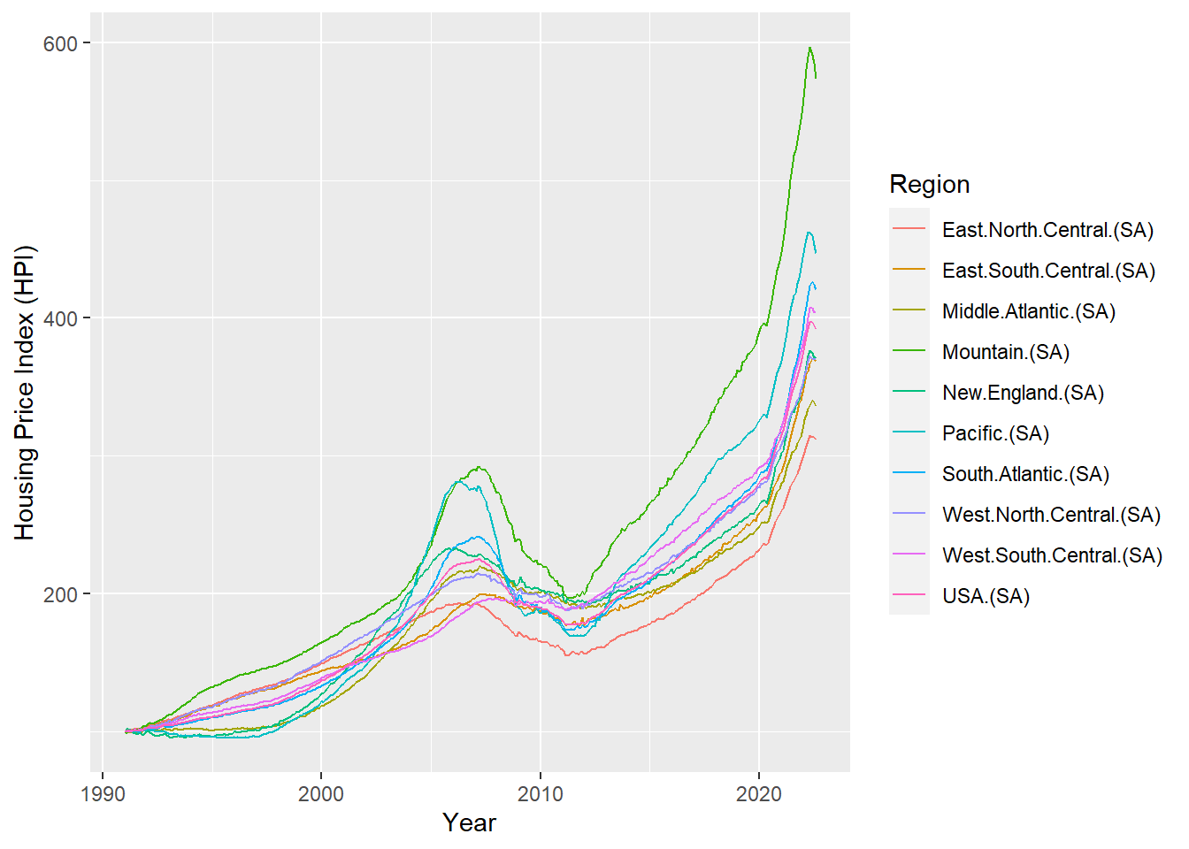

# All sa data polar plot
ggplot(sa_hpi, aes(x = Month, 
                   y = value,
                   group = variable, color = variable)) +
  geom_line() +
  coord_polar() +
  xlab("Year") + ylab("Housing Price Index (HPI)") +
  labs(color = "Region") +
  facet_wrap(~variable)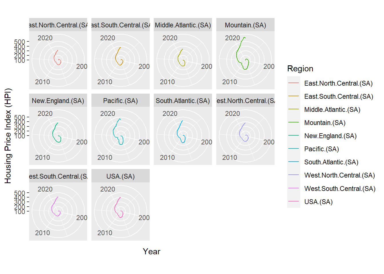

# Line plot by specific year
# Replace "1991" with input year
ggplot(sa_hpi %>% filter(grepl("1991", Month)), 
       aes(x = Month, y = value,
        group = variable, color = variable)) +
  geom_line() +
  xlab("Month") + ylab("Housing Price Index (HPI)") +
  labs(color = "Region")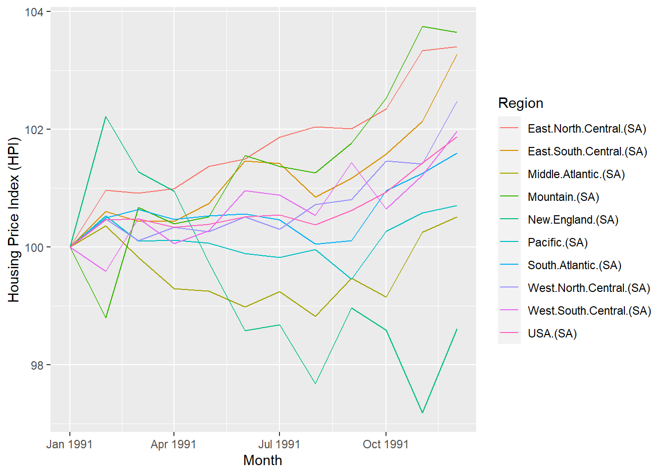

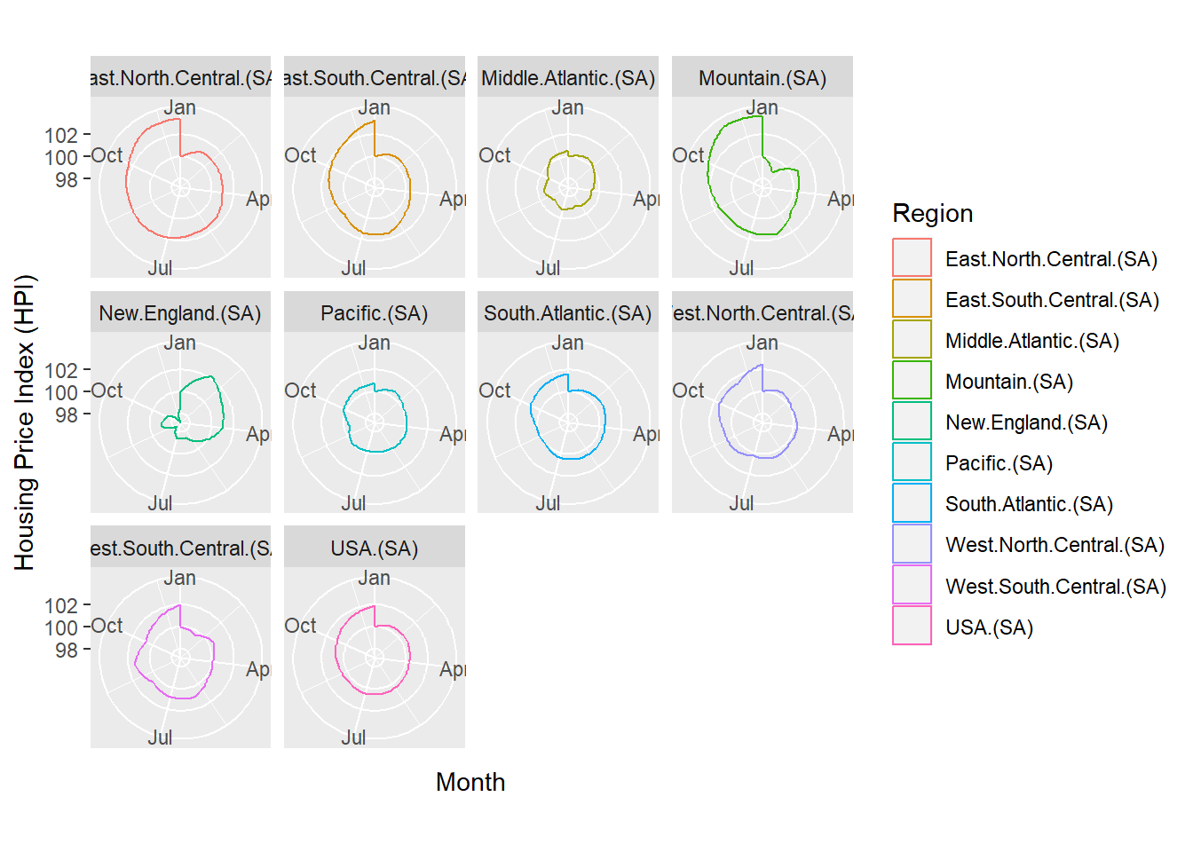
# Facet wrapped polar grids by specific year
# Replace "1991" with input year
ggplot(sa_hpi %>% filter(grepl("1991", Month)), 
       aes(x = Month, y = value,
           group = variable, color = variable)) +
  geom_polygon(fill = NA) +
  coord_polar() +
  facet_wrap(~variable) +
  xlab("Month") + ylab("Housing Price Index (HPI)") +
  labs(color = "Region")

Code used to build Shiny App

library(tidyverse)
library(shiny)
library(openxlsx)
library(reshape2)

# Loading & wrangling data

hpi <- read.xlsx(xlsxFile = "https://github.com/aldenfelix/aldenfelix.github.io/raw/main/Data/HPI_PO_monthly_hist.xlsx", 
                 startRow = 4, 
                 detectDates = TRUE)

# Select seasonally adjusted variables
# NOTE: TO INCLUDE PARENTHESES IN SEARCH USE \\ AS SEEN BELOW
sa_vars <- hpi %>% 
  select(grep("\\(SA\\)|Month", colnames(hpi)))

# Turn data from wide to long format for time series using reshape2 library
sa_hpi <- melt(sa_vars, id.vars = "Month")



# Define UI for app ----
ui <- fluidPage(
  
  # App title ----
  titlePanel("Federal Housing Finance Agency Housing Price Index (FHFA HPI)"),
  
  # Sidebar layout with input and output definitions ----
  sidebarLayout(
    
    # Sidebar panel for inputs ----
    sidebarPanel(
      
      # Input: Buttons for type of plot
      radioButtons(inputId = "plotbtn",
                   label = "Choose what kind of plot to create",
                   choices = c("Line plot for a specific year" = "lineyear", 
                               "Polar plot for a specific year" = "polar",
                               "Line plot of all data" = "line")),
      
      # Input: Slider for year, conditional on plots where time can be specified
      conditionalPanel(
        condition = "input.plotbtn == 'lineyear' || input.plotbtn == 'polar'", 
        sliderInput(inputId = "year",
                  label = "Choose a year to view:",
                  min = 1991,
                  max = 2022,
                  value = 1991)),
      
      # Input: Slider for number of observations
      sliderInput(inputId = "obs",
                  label = "Number of observations:",
                  min = 1,
                  max = 48,
                  value = 24),
    ),
    
    # Main panel for displaying outputs ----
    mainPanel(
      
      # Output: Panel that displays line plot
      conditionalPanel(
        condition = "input.plotbtn == 'lineyear'",
        plotOutput(width = 1000, height = 1000, "lineplotyear")
      ),
      
      # Output: Panel that displays polar plot
      conditionalPanel(
        condition = "input.plotbtn == 'polar'",
        plotOutput(width = 1500, height = 1500, "polarplot")
      ),
      
      # Output: Panel that displays line plot of all data
      conditionalPanel(
        condition = "input.plotbtn == 'line'",
        plotOutput(width = 1000, height = 1000, "lineplot")
      ),
      
      # Output: Verbatim text for data summary ----
      verbatimTextOutput("summary"),
      
      # Output: HTML table with requested number of observations ----
      tableOutput("obs")
      
      # Output: Formatted text for caption ----
      # h3(textOutput("caption", container = span)),
    )
  )
)

# Define server logic to summarize and view selected dataset ----
server <- function(input, output) {
  
  output$summary <- renderPrint({
    summary(hpi)
  })
  
  # Show the first "n" observations ----
  # The output$view depends on both the databaseInput reactive
  # expression and input$obs, so it will be re-executed whenever
  # input$dataset or input$obs is changed
  output$obs <- renderTable({
    hpi$Month <- as.character(as.Date(hpi$Month, "%Y-%m-%d"))
    head(hpi, n = input$obs)
  })
  
  output$lineplotyear <- renderPlot({
    ggplot(sa_hpi %>% filter(grepl(as.character(input$year), Month)), 
           aes(x = Month, y = value,
           group = variable, color = variable)) +
      geom_line(size = 1.1) +
      xlab("Month") + ylab("Housing Price Index (HPI)") +
      labs(color = "Region") +
      scale_x_date(breaks = "month", labels = scales::label_date("%b")) +
      theme(text = element_text(size = 20))
  })

  output$polarplot <- renderPlot({
    ggplot(sa_hpi %>% filter(grepl(as.character(input$year), Month)), 
           aes(x = Month, y = value,
               group = variable, color = variable)) +
      geom_polygon(fill = NA, size = 1.1) +
      coord_polar() +
      facet_wrap(~variable) +
      xlab("Month") + ylab("Housing Price Index (HPI)") +
      labs(color = "Region") +
      scale_x_date(breaks = "month", labels = scales::label_date("%b")) +
      theme(text = element_text(size = 20))
  })
  
  output$lineplot <- renderPlot({
    ggplot(sa_hpi, aes(x = Month, y = value,
                       group = variable, 
                       color = variable)) +
      xlab("Year") + ylab("Housing Price Index (HPI)") +
      labs(color = "Region") +
      geom_line(size = 1.05) +
      xlab("Year") + ylab("Housing Price Index (HPI)") +
      labs(color = "Region") +
      theme(text = element_text(size = 20))
  })
}

# Create Shiny app ----
shinyApp(ui, server)

Shiny applications not supported in static R Markdown documents