EPPS 6323 Assignment 6

Linear Regression

# Knowledge Mining: Linear regression
# File: Lab_linearregression01.R
# Theme: Linear regression
# Data: MASS, ISLR
# Adapted from ISLR Chapter 3 Lab

#install.packages(c("easypackages","MASS","ISLR","arm"))
library(easypackages)
libraries("arm","MASS","ISLR")

## Load datasets from MASS and ISLR packages
attach(Boston)

### Simple linear regression
names(Boston)

 [1] "crim"    "zn"      "indus"   "chas"    "nox"     "rm"      "age"    
 [8] "dis"     "rad"     "tax"     "ptratio" "black"   "lstat"   "medv"   

# What is the Boston dataset?
#?Boston
plot(medv~lstat,Boston, pch=20, cex=.8, col="steelblue")
fit1=lm(medv~lstat,data=Boston)
fit1

Call:
lm(formula = medv ~ lstat, data = Boston)

Coefficients:
(Intercept)        lstat  
      34.55        -0.95  

summary(fit1)

Call:
lm(formula = medv ~ lstat, data = Boston)

Residuals:
    Min      1Q  Median      3Q     Max 
-15.168  -3.990  -1.318   2.034  24.500 

Coefficients:
            Estimate Std. Error t value Pr(>|t|)    
(Intercept) 34.55384    0.56263   61.41   <2e-16 ***
lstat       -0.95005    0.03873  -24.53   <2e-16 ***
---
Signif. codes:  0 '***' 0.001 '**' 0.01 '*' 0.05 '.' 0.1 ' ' 1

Residual standard error: 6.216 on 504 degrees of freedom
Multiple R-squared:  0.5441,    Adjusted R-squared:  0.5432 
F-statistic: 601.6 on 1 and 504 DF,  p-value: < 2.2e-16

abline(fit1,col="firebrick")

names(fit1)

 [1] "coefficients"  "residuals"     "effects"       "rank"         
 [5] "fitted.values" "assign"        "qr"            "df.residual"  
 [9] "xlevels"       "call"          "terms"         "model"        

confint(fit1) # confidence intervals

                2.5 %     97.5 %
(Intercept) 33.448457 35.6592247
lstat       -1.026148 -0.8739505

# Predictions using values in lstat
predict(fit1,data.frame(lstat=c(0,5,10,15)),interval="confidence") # confidence intervals

       fit      lwr      upr
1 34.55384 33.44846 35.65922
2 29.80359 29.00741 30.59978
3 25.05335 24.47413 25.63256
4 20.30310 19.73159 20.87461

predict(fit1,data.frame(lstat=c(0,5,10,15)),interval="prediction") # prediction intervals

       fit       lwr      upr
1 34.55384 22.291923 46.81576
2 29.80359 17.565675 42.04151
3 25.05335 12.827626 37.27907
4 20.30310  8.077742 32.52846

# Prediction interval uses sample mean and takes into account the variability of the estimators for μ and σ.
# Therefore, the interval will be wider.

### Multiple linear regression
fit2=lm(medv~lstat+age,data=Boston)
summary(fit2)

Call:
lm(formula = medv ~ lstat + age, data = Boston)

Residuals:
    Min      1Q  Median      3Q     Max 
-15.981  -3.978  -1.283   1.968  23.158 

Coefficients:
            Estimate Std. Error t value Pr(>|t|)    
(Intercept) 33.22276    0.73085  45.458  < 2e-16 ***
lstat       -1.03207    0.04819 -21.416  < 2e-16 ***
age          0.03454    0.01223   2.826  0.00491 ** 
---
Signif. codes:  0 '***' 0.001 '**' 0.01 '*' 0.05 '.' 0.1 ' ' 1

Residual standard error: 6.173 on 503 degrees of freedom
Multiple R-squared:  0.5513,    Adjusted R-squared:  0.5495 
F-statistic:   309 on 2 and 503 DF,  p-value: < 2.2e-16

fit3=lm(medv~.,Boston)
summary(fit3)

Call:
lm(formula = medv ~ ., data = Boston)

Residuals:
    Min      1Q  Median      3Q     Max 
-15.595  -2.730  -0.518   1.777  26.199 

Coefficients:
              Estimate Std. Error t value Pr(>|t|)    
(Intercept)  3.646e+01  5.103e+00   7.144 3.28e-12 ***
crim        -1.080e-01  3.286e-02  -3.287 0.001087 ** 
zn           4.642e-02  1.373e-02   3.382 0.000778 ***
indus        2.056e-02  6.150e-02   0.334 0.738288    
chas         2.687e+00  8.616e-01   3.118 0.001925 ** 
nox         -1.777e+01  3.820e+00  -4.651 4.25e-06 ***
rm           3.810e+00  4.179e-01   9.116  < 2e-16 ***
age          6.922e-04  1.321e-02   0.052 0.958229    
dis         -1.476e+00  1.995e-01  -7.398 6.01e-13 ***
rad          3.060e-01  6.635e-02   4.613 5.07e-06 ***
tax         -1.233e-02  3.760e-03  -3.280 0.001112 ** 
ptratio     -9.527e-01  1.308e-01  -7.283 1.31e-12 ***
black        9.312e-03  2.686e-03   3.467 0.000573 ***
lstat       -5.248e-01  5.072e-02 -10.347  < 2e-16 ***
---
Signif. codes:  0 '***' 0.001 '**' 0.01 '*' 0.05 '.' 0.1 ' ' 1

Residual standard error: 4.745 on 492 degrees of freedom
Multiple R-squared:  0.7406,    Adjusted R-squared:  0.7338 
F-statistic: 108.1 on 13 and 492 DF,  p-value: < 2.2e-16

par(mfrow=c(2,2))
plot(fit3,pch=20, cex=.8, col="steelblue")
mtext("fit3", side = 3, line = - 2, cex = 2, outer = TRUE)

# Update function to re-specify the model, i.e. include all but age and indus variables
fit4=update(fit3,~.-age-indus)
summary(fit4)

Call:
lm(formula = medv ~ crim + zn + chas + nox + rm + dis + rad + 
    tax + ptratio + black + lstat, data = Boston)

Residuals:
     Min       1Q   Median       3Q      Max 
-15.5984  -2.7386  -0.5046   1.7273  26.2373 

Coefficients:
              Estimate Std. Error t value Pr(>|t|)    
(Intercept)  36.341145   5.067492   7.171 2.73e-12 ***
crim         -0.108413   0.032779  -3.307 0.001010 ** 
zn            0.045845   0.013523   3.390 0.000754 ***
chas          2.718716   0.854240   3.183 0.001551 ** 
nox         -17.376023   3.535243  -4.915 1.21e-06 ***
rm            3.801579   0.406316   9.356  < 2e-16 ***
dis          -1.492711   0.185731  -8.037 6.84e-15 ***
rad           0.299608   0.063402   4.726 3.00e-06 ***
tax          -0.011778   0.003372  -3.493 0.000521 ***
ptratio      -0.946525   0.129066  -7.334 9.24e-13 ***
black         0.009291   0.002674   3.475 0.000557 ***
lstat        -0.522553   0.047424 -11.019  < 2e-16 ***
---
Signif. codes:  0 '***' 0.001 '**' 0.01 '*' 0.05 '.' 0.1 ' ' 1

Residual standard error: 4.736 on 494 degrees of freedom
Multiple R-squared:  0.7406,    Adjusted R-squared:  0.7348 
F-statistic: 128.2 on 11 and 494 DF,  p-value: < 2.2e-16

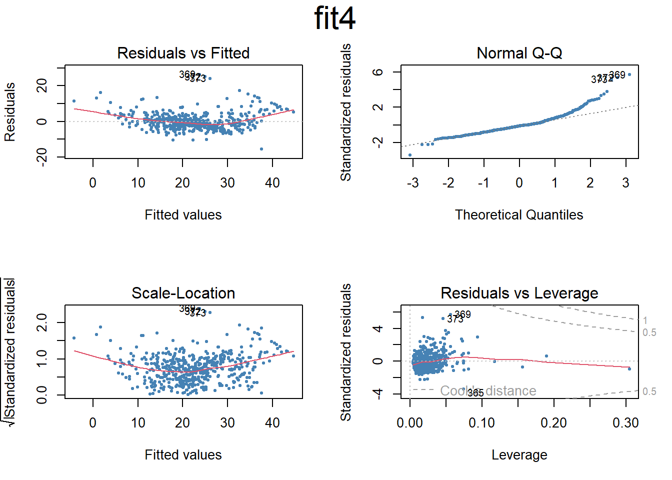
# Set the next plot configuration
par(mfrow=c(2,2), main="fit4")
plot(fit4,pch=20, cex=.8, col="steelblue")
mtext("fit4", side = 3, line = - 2, cex = 2, outer = TRUE)

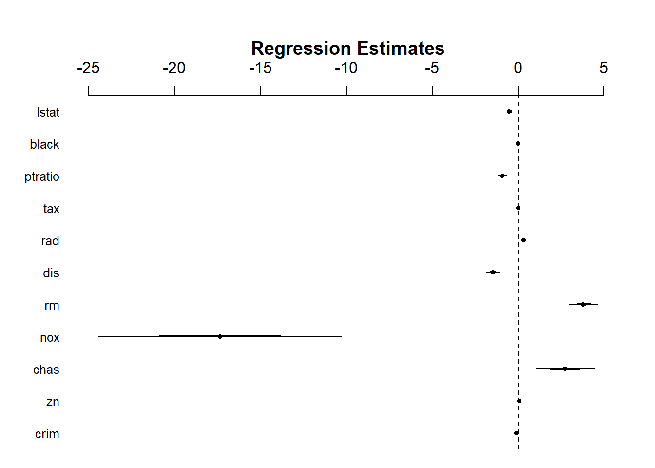
# Uses coefplot to plot coefficients.  Note the line at 0.
par(mfrow=c(1,1))
arm::coefplot(fit4)

### Nonlinear terms and Interactions
fit5=lm(medv~lstat*age,Boston) # include both variables and the interaction term x1:x2
summary(fit5)

Call:
lm(formula = medv ~ lstat * age, data = Boston)

Residuals:
    Min      1Q  Median      3Q     Max 
-15.806  -4.045  -1.333   2.085  27.552 

Coefficients:
              Estimate Std. Error t value Pr(>|t|)    
(Intercept) 36.0885359  1.4698355  24.553  < 2e-16 ***
lstat       -1.3921168  0.1674555  -8.313 8.78e-16 ***
age         -0.0007209  0.0198792  -0.036   0.9711    
lstat:age    0.0041560  0.0018518   2.244   0.0252 *  
---
Signif. codes:  0 '***' 0.001 '**' 0.01 '*' 0.05 '.' 0.1 ' ' 1

Residual standard error: 6.149 on 502 degrees of freedom
Multiple R-squared:  0.5557,    Adjusted R-squared:  0.5531 
F-statistic: 209.3 on 3 and 502 DF,  p-value: < 2.2e-16

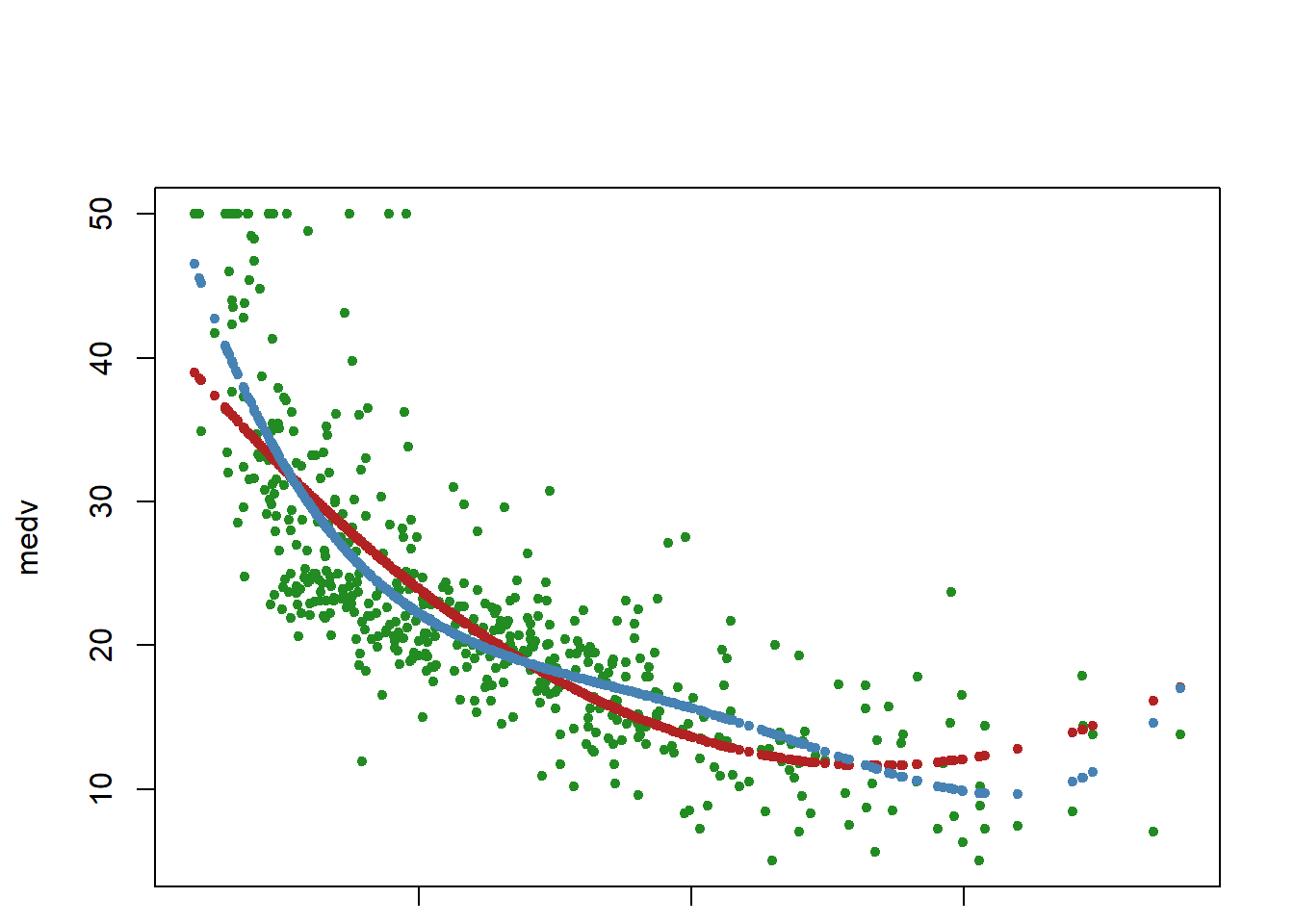
## I() identity function for squared term to interpret as-is
## Combine two command lines with semicolon
fit6=lm(medv~lstat +I(lstat^2),Boston); summary(fit6)

Call:
lm(formula = medv ~ lstat + I(lstat^2), data = Boston)

Residuals:
     Min       1Q   Median       3Q      Max 
-15.2834  -3.8313  -0.5295   2.3095  25.4148 

Coefficients:
             Estimate Std. Error t value Pr(>|t|)    
(Intercept) 42.862007   0.872084   49.15   <2e-16 ***
lstat       -2.332821   0.123803  -18.84   <2e-16 ***
I(lstat^2)   0.043547   0.003745   11.63   <2e-16 ***
---
Signif. codes:  0 '***' 0.001 '**' 0.01 '*' 0.05 '.' 0.1 ' ' 1

Residual standard error: 5.524 on 503 degrees of freedom
Multiple R-squared:  0.6407,    Adjusted R-squared:  0.6393 
F-statistic: 448.5 on 2 and 503 DF,  p-value: < 2.2e-16

par(mfrow=c(1,1))
plot(medv~lstat, pch=20, col="forestgreen")

points(lstat,fitted(fit6),col="firebrick",pch=20)
fit7=lm(medv~poly(lstat,4))
points(lstat,fitted(fit7),col="steelblue",pch=20)

###Qualitative predictors
names(Carseats)

 [1] "Sales"       "CompPrice"   "Income"      "Advertising" "Population" 
 [6] "Price"       "ShelveLoc"   "Age"         "Education"   "Urban"      
[11] "US"         

summary(Carseats)

     Sales          CompPrice       Income        Advertising    
 Min.   : 0.000   Min.   : 77   Min.   : 21.00   Min.   : 0.000  
 1st Qu.: 5.390   1st Qu.:115   1st Qu.: 42.75   1st Qu.: 0.000  
 Median : 7.490   Median :125   Median : 69.00   Median : 5.000  
 Mean   : 7.496   Mean   :125   Mean   : 68.66   Mean   : 6.635  
 3rd Qu.: 9.320   3rd Qu.:135   3rd Qu.: 91.00   3rd Qu.:12.000  
 Max.   :16.270   Max.   :175   Max.   :120.00   Max.   :29.000  
   Population        Price        ShelveLoc        Age          Education   
 Min.   : 10.0   Min.   : 24.0   Bad   : 96   Min.   :25.00   Min.   :10.0  
 1st Qu.:139.0   1st Qu.:100.0   Good  : 85   1st Qu.:39.75   1st Qu.:12.0  
 Median :272.0   Median :117.0   Medium:219   Median :54.50   Median :14.0  
 Mean   :264.8   Mean   :115.8                Mean   :53.32   Mean   :13.9  
 3rd Qu.:398.5   3rd Qu.:131.0                3rd Qu.:66.00   3rd Qu.:16.0  
 Max.   :509.0   Max.   :191.0                Max.   :80.00   Max.   :18.0  
 Urban       US     
 No :118   No :142  
 Yes:282   Yes:258  
                    
                    
                    
                    

fit1=lm(Sales~.+Income:Advertising+Age:Price,Carseats) # add two interaction terms
summary(fit1)

Call:
lm(formula = Sales ~ . + Income:Advertising + Age:Price, data = Carseats)

Residuals:
    Min      1Q  Median      3Q     Max 
-2.9208 -0.7503  0.0177  0.6754  3.3413 

Coefficients:
                     Estimate Std. Error t value Pr(>|t|)    
(Intercept)         6.5755654  1.0087470   6.519 2.22e-10 ***
CompPrice           0.0929371  0.0041183  22.567  < 2e-16 ***
Income              0.0108940  0.0026044   4.183 3.57e-05 ***
Advertising         0.0702462  0.0226091   3.107 0.002030 ** 
Population          0.0001592  0.0003679   0.433 0.665330    
Price              -0.1008064  0.0074399 -13.549  < 2e-16 ***
ShelveLocGood       4.8486762  0.1528378  31.724  < 2e-16 ***
ShelveLocMedium     1.9532620  0.1257682  15.531  < 2e-16 ***
Age                -0.0579466  0.0159506  -3.633 0.000318 ***
Education          -0.0208525  0.0196131  -1.063 0.288361    
UrbanYes            0.1401597  0.1124019   1.247 0.213171    
USYes              -0.1575571  0.1489234  -1.058 0.290729    
Income:Advertising  0.0007510  0.0002784   2.698 0.007290 ** 
Price:Age           0.0001068  0.0001333   0.801 0.423812    
---
Signif. codes:  0 '***' 0.001 '**' 0.01 '*' 0.05 '.' 0.1 ' ' 1

Residual standard error: 1.011 on 386 degrees of freedom
Multiple R-squared:  0.8761,    Adjusted R-squared:  0.8719 
F-statistic:   210 on 13 and 386 DF,  p-value: < 2.2e-16

attach(Carseats)
contrasts(Carseats$ShelveLoc) # what is contrasts function?

       Good Medium
Bad       0      0
Good      1      0
Medium    0      1

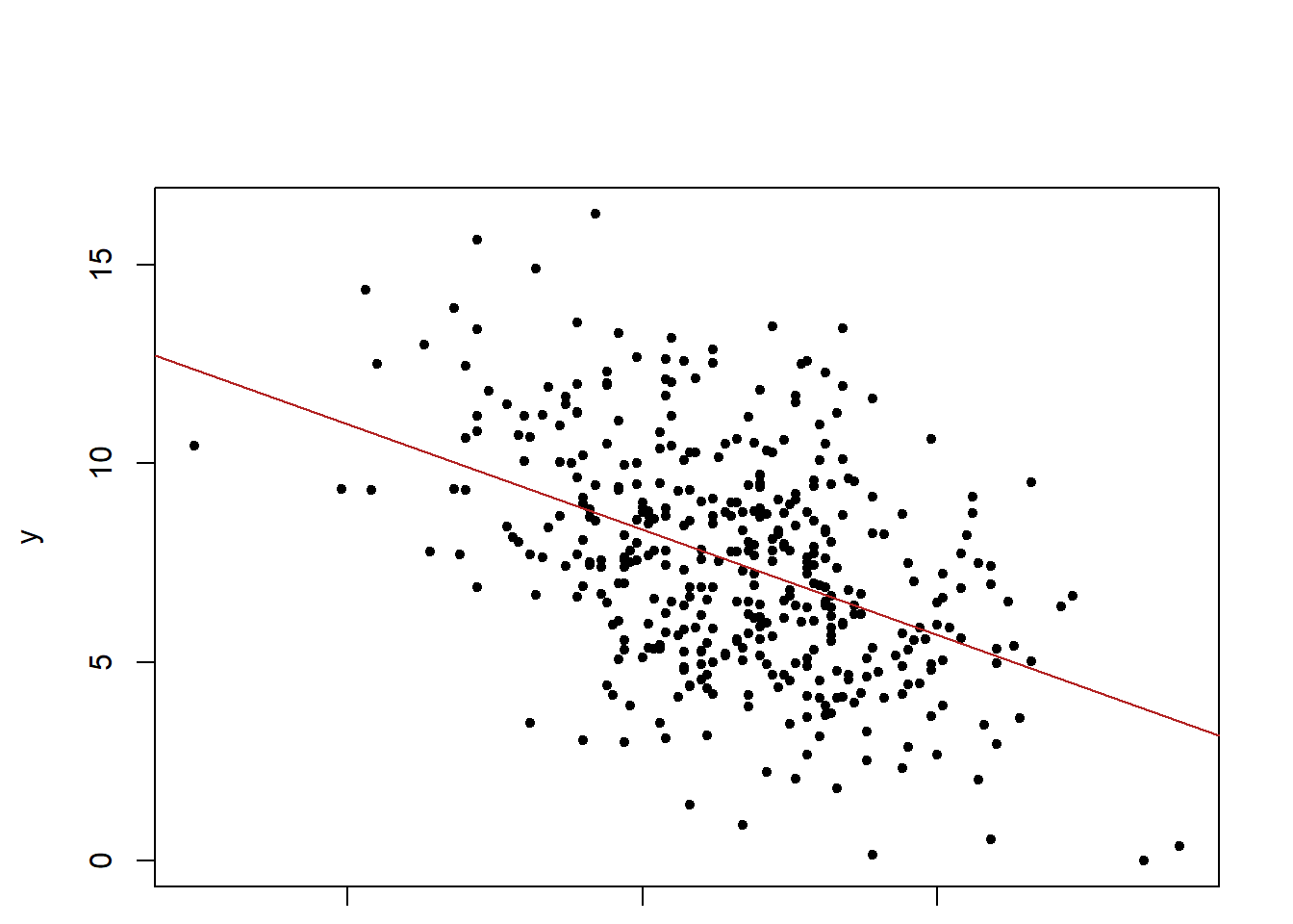
#?contrasts

### Writing an R function to combine the lm, plot and abline functions to 
### create a one step regression fit plot function
regplot=function(x,y){
  fit=lm(y~x)
  plot(x,y, pch=20)
  abline(fit,col="firebrick")
}
attach(Carseats)
regplot(Price,Sales)

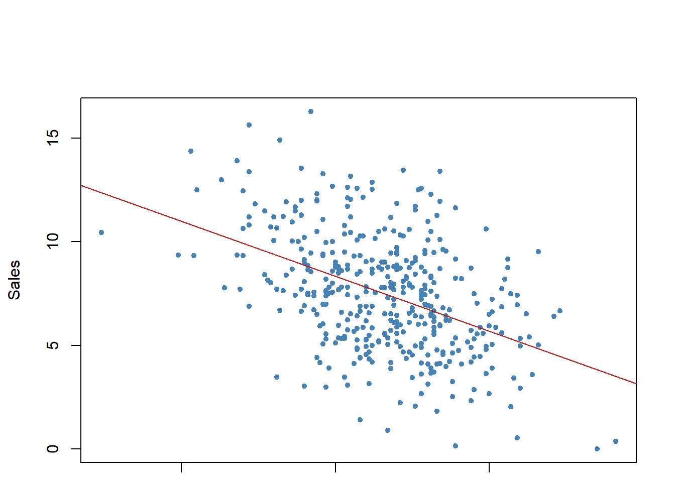
## Allow extra room for additional arguments/specifications
regplot=function(x,y,...){
  fit=lm(y~x)
  plot(x,y,...)
  abline(fit,col="firebrick")
}
regplot(Price,Sales,xlab="Price",ylab="Sales",col="steelblue",pch=20)

## Additional note: try out the coefplot2 package to finetune the coefplots
##install.packages("coefplot2", repos="http://www.math.mcmaster.ca/bolker/R", type="source")
## library(coefplot2)

# Exercise 
# Try other combination of interactive terms
# How to interpret interactive terms?
# Read: Brambor, T., Clark, W.R. and Golder, M., 2006. Understanding interaction models: Improving empirical analyses. Political analysis, 14(1), pp.63-82.
# What are qualitative variables?  What class should they be? 

TEDS2016 Dataset

library(haven) 
TEDS_2016 <- read_stata("https://github.com/datageneration/home/blob/master/DataProgramming/data/TEDS_2016.dta?raw=true")

glm.vt=glm(votetsai~female, data=TEDS_2016,family=binomial)
summary(glm.vt)

Call:
glm(formula = votetsai ~ female, family = binomial, data = TEDS_2016)

Deviance Residuals: 
    Min       1Q   Median       3Q      Max  
-1.4180  -1.3889   0.9546   0.9797   0.9797  

Coefficients:
            Estimate Std. Error z value Pr(>|z|)    
(Intercept)  0.54971    0.08245   6.667 2.61e-11 ***
female      -0.06517    0.11644  -0.560    0.576    
---
Signif. codes:  0 '***' 0.001 '**' 0.01 '*' 0.05 '.' 0.1 ' ' 1

(Dispersion parameter for binomial family taken to be 1)

    Null deviance: 1666.5  on 1260  degrees of freedom
Residual deviance: 1666.2  on 1259  degrees of freedom
  (429 observations deleted due to missingness)
AIC: 1670.2

Number of Fisher Scoring iterations: 4

glm.vt2=glm(votetsai~female + KMT + DPP + age + edu + income, 
            data=TEDS_2016,family=binomial)
summary(glm.vt2)

Call:
glm(formula = votetsai ~ female + KMT + DPP + age + edu + income, 
    family = binomial, data = TEDS_2016)

Deviance Residuals: 
    Min       1Q   Median       3Q      Max  
-2.7360  -0.3673   0.2408   0.2946   2.5408  

Coefficients:
             Estimate Std. Error z value Pr(>|z|)    
(Intercept)  1.618640   0.592084   2.734  0.00626 ** 
female       0.047406   0.177403   0.267  0.78930    
KMT         -3.156273   0.250360 -12.607  < 2e-16 ***
DPP          2.888943   0.267968  10.781  < 2e-16 ***
age         -0.011808   0.007164  -1.648  0.09931 .  
edu         -0.184604   0.083102  -2.221  0.02632 *  
income       0.013727   0.034382   0.399  0.68971    
---
Signif. codes:  0 '***' 0.001 '**' 0.01 '*' 0.05 '.' 0.1 ' ' 1

(Dispersion parameter for binomial family taken to be 1)

    Null deviance: 1661.76  on 1256  degrees of freedom
Residual deviance:  836.15  on 1250  degrees of freedom
  (433 observations deleted due to missingness)
AIC: 850.15

Number of Fisher Scoring iterations: 6

glm.vt3=glm(votetsai~female + KMT + DPP + age + edu + income +
              Independence + Econ_worse + Govt_dont_care + 
              Minnan_father + Mainland_father + Taiwanese, 
            data=TEDS_2016,family=binomial)
summary(glm.vt3)

Call:
glm(formula = votetsai ~ female + KMT + DPP + age + edu + income + 
    Independence + Econ_worse + Govt_dont_care + Minnan_father + 
    Mainland_father + Taiwanese, family = binomial, data = TEDS_2016)

Deviance Residuals: 
    Min       1Q   Median       3Q      Max  
-3.1060  -0.3143   0.1744   0.3975   2.7917  

Coefficients:
                 Estimate Std. Error z value Pr(>|z|)    
(Intercept)     -0.015976   0.679780  -0.024  0.98125    
female          -0.097996   0.189840  -0.516  0.60571    
KMT             -2.922246   0.259333 -11.268  < 2e-16 ***
DPP              2.468855   0.275350   8.966  < 2e-16 ***
age              0.003287   0.007884   0.417  0.67672    
edu             -0.092110   0.090119  -1.022  0.30674    
income           0.021771   0.036406   0.598  0.54984    
Independence     1.020953   0.251776   4.055 5.01e-05 ***
Econ_worse       0.310462   0.189100   1.642  0.10063    
Govt_dont_care  -0.014295   0.188765  -0.076  0.93964    
Minnan_father   -0.247650   0.253921  -0.975  0.32941    
Mainland_father -1.089332   0.396822  -2.745  0.00605 ** 
Taiwanese        0.909019   0.198930   4.570 4.89e-06 ***
---
Signif. codes:  0 '***' 0.001 '**' 0.01 '*' 0.05 '.' 0.1 ' ' 1

(Dispersion parameter for binomial family taken to be 1)

    Null deviance: 1661.76  on 1256  degrees of freedom
Residual deviance:  767.13  on 1244  degrees of freedom
  (433 observations deleted due to missingness)
AIC: 793.13

Number of Fisher Scoring iterations: 6