x <- c(1,3,2,5)
x
[1] 1 3 2 5x = c(1,6,2)
x[1] 1 6 2y = c(1,4,3)x <- c(1,3,2,5)
x[1] 1 3 2 5x = c(1,6,2)
x[1] 1 6 2y = c(1,4,3)length(x) # What does length() do?[1] 3length(y)[1] 3x+y[1] 2 10 5ls() # List objects in the environment[1] "has_annotations" "x" "y" rm(x,y) # Remove objects
ls()[1] "has_annotations"rm(list=ls()) # Danger! What does this do? Not recommended!#?matrix
x=matrix(data=c(1,2,3,4), nrow=2, ncol=2) # Create a 2x2 matrix object
x [,1] [,2]
[1,] 1 3
[2,] 2 4x=matrix(c(1,2,3,4),2,2)
matrix(c(1,2,3,4),2,2,byrow=TRUE) # What about byrow=F? [,1] [,2]
[1,] 1 2
[2,] 3 4sqrt(x) # What does x look like? [,1] [,2]
[1,] 1.000000 1.732051
[2,] 1.414214 2.000000x^2 [,1] [,2]
[1,] 1 9
[2,] 4 16x=rnorm(50) # Generate a vector of 50 numbers using the rnorm() function
y=x+rnorm(50,mean=50,sd=.1) # What does rnorm(50,mean=50,sd=.1) generate?
cor(x,y) # Correlation of x and y[1] 0.9977306set.seed(1303) # Set the seed for Random Number Generator (RNG) to generate values that are reproducible.
rnorm(50) [1] -1.1439763145 1.3421293656 2.1853904757 0.5363925179 0.0631929665
[6] 0.5022344825 -0.0004167247 0.5658198405 -0.5725226890 -1.1102250073
[11] -0.0486871234 -0.6956562176 0.8289174803 0.2066528551 -0.2356745091
[16] -0.5563104914 -0.3647543571 0.8623550343 -0.6307715354 0.3136021252
[21] -0.9314953177 0.8238676185 0.5233707021 0.7069214120 0.4202043256
[26] -0.2690521547 -1.5103172999 -0.6902124766 -0.1434719524 -1.0135274099
[31] 1.5732737361 0.0127465055 0.8726470499 0.4220661905 -0.0188157917
[36] 2.6157489689 -0.6931401748 -0.2663217810 -0.7206364412 1.3677342065
[41] 0.2640073322 0.6321868074 -1.3306509858 0.0268888182 1.0406363208
[46] 1.3120237985 -0.0300020767 -0.2500257125 0.0234144857 1.6598706557set.seed(3) # Try different seeds?
y=rnorm(100)mean(y)[1] 0.01103557var(y)[1] 0.7328675sqrt(var(y))[1] 0.8560768sd(y)[1] 0.8560768x=rnorm(100)
y=rnorm(100)
plot(x,y, pch=20, col = "blue") # Scatterplot for two numeric variables by default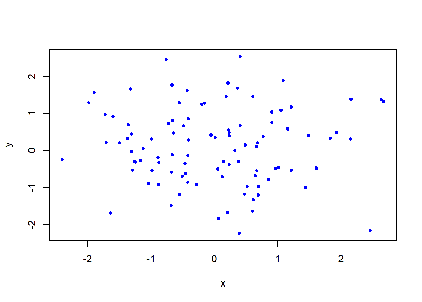
plot(x,y, pch=20, col = "blue",xlab="this is the x-axis",ylab="this is the y-axis",main="Plot of X vs Y") # Add labels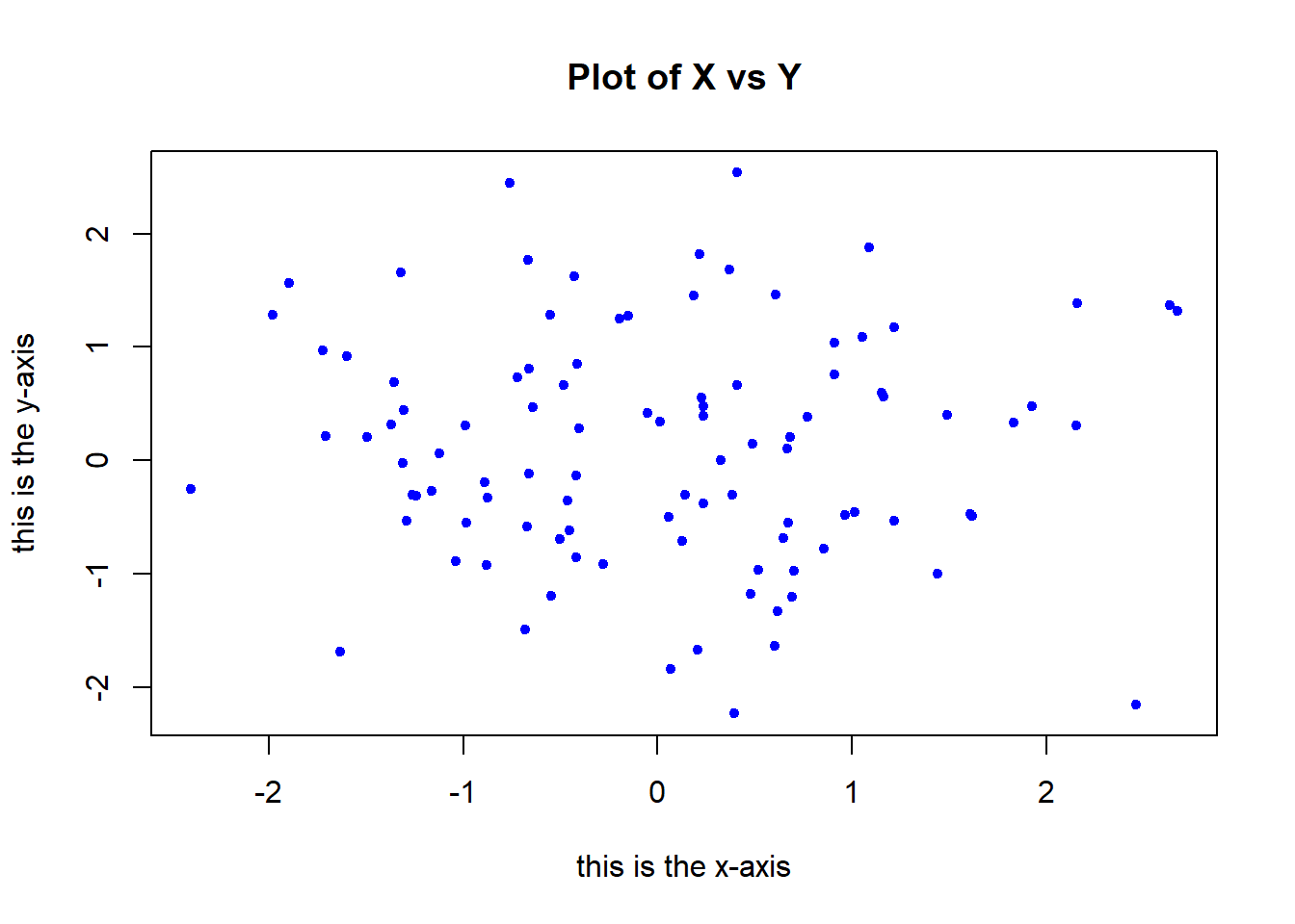
pdf("Figure01.pdf") # Save as pdf, add a path or it will be stored on the project directory
plot(x,y,pch=20, col="forestgreen") # Try different colors?
dev.off() # Close the file using the dev.off function
png
2 x=seq(1,10) # Same as x=c(1:10)
x [1] 1 2 3 4 5 6 7 8 9 10x=1:10
x [1] 1 2 3 4 5 6 7 8 9 10x=seq(-pi,pi,length=50)
y=x(Adapted from ISLR Chapter 3 Lab: Introduction to R)
A=matrix(1:16,4,4)
A
[,1] [,2] [,3] [,4]
[1,] 1 5 9 13
[2,] 2 6 10 14
[3,] 3 7 11 15
[4,] 4 8 12 16A[2,3][1] 10A[c(1,3),c(2,4)] [,1] [,2]
[1,] 5 13
[2,] 7 15A[1:3,2:4] [,1] [,2] [,3]
[1,] 5 9 13
[2,] 6 10 14
[3,] 7 11 15A[1:2,] [,1] [,2] [,3] [,4]
[1,] 1 5 9 13
[2,] 2 6 10 14A[,1:2] [,1] [,2]
[1,] 1 5
[2,] 2 6
[3,] 3 7
[4,] 4 8A[1,][1] 1 5 9 13A[-c(1,3),] [,1] [,2] [,3] [,4]
[1,] 2 6 10 14
[2,] 4 8 12 16A[-c(1,3),-c(1,3,4)][1] 6 8dim(A)[1] 4 4Auto=read.table("https://raw.githubusercontent.com/karlho/knowledgemining/gh-pages/data/Auto.data")
# fix(Auto) # Starting the X11 R data editor
Auto=read.table("https://raw.githubusercontent.com/karlho/knowledgemining/gh-pages/data/Auto.data",header=T,na.strings="?")
# fix(Auto)
Auto=read.csv("https://raw.githubusercontent.com/karlho/knowledgemining/gh-pages/data/Auto.csv",header=T,na.strings="?")
# fix(Auto)
dim(Auto)[1] 397 9Auto[1:4,] mpg cylinders displacement horsepower weight acceleration year origin
1 18 8 307 130 3504 12.0 70 1
2 15 8 350 165 3693 11.5 70 1
3 18 8 318 150 3436 11.0 70 1
4 16 8 304 150 3433 12.0 70 1
name
1 chevrolet chevelle malibu
2 buick skylark 320
3 plymouth satellite
4 amc rebel sstAuto=na.omit(Auto)
dim(Auto)[1] 392 9names(Auto)[1] "mpg" "cylinders" "displacement" "horsepower" "weight"
[6] "acceleration" "year" "origin" "name" Auto=read.table("https://www.statlearning.com/s/Auto.data",header=T,na.strings="?")
dim(Auto)[1] 397 9# plot(cylinders, mpg)
plot(Auto$cylinders, Auto$mpg)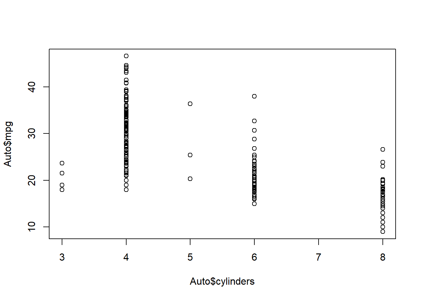
attach(Auto)
plot(cylinders, mpg)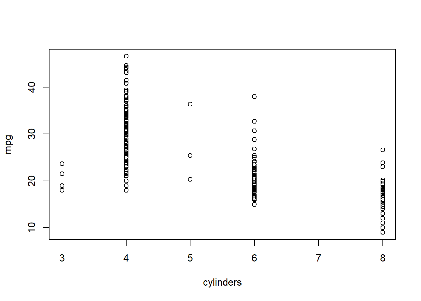
cylinders=as.factor(cylinders)
plot(cylinders, mpg)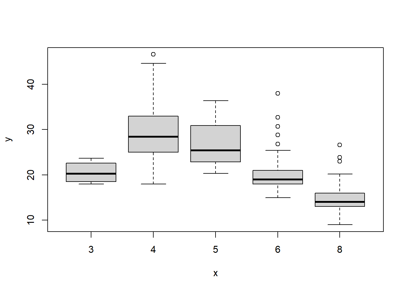
plot(cylinders, mpg, col="red")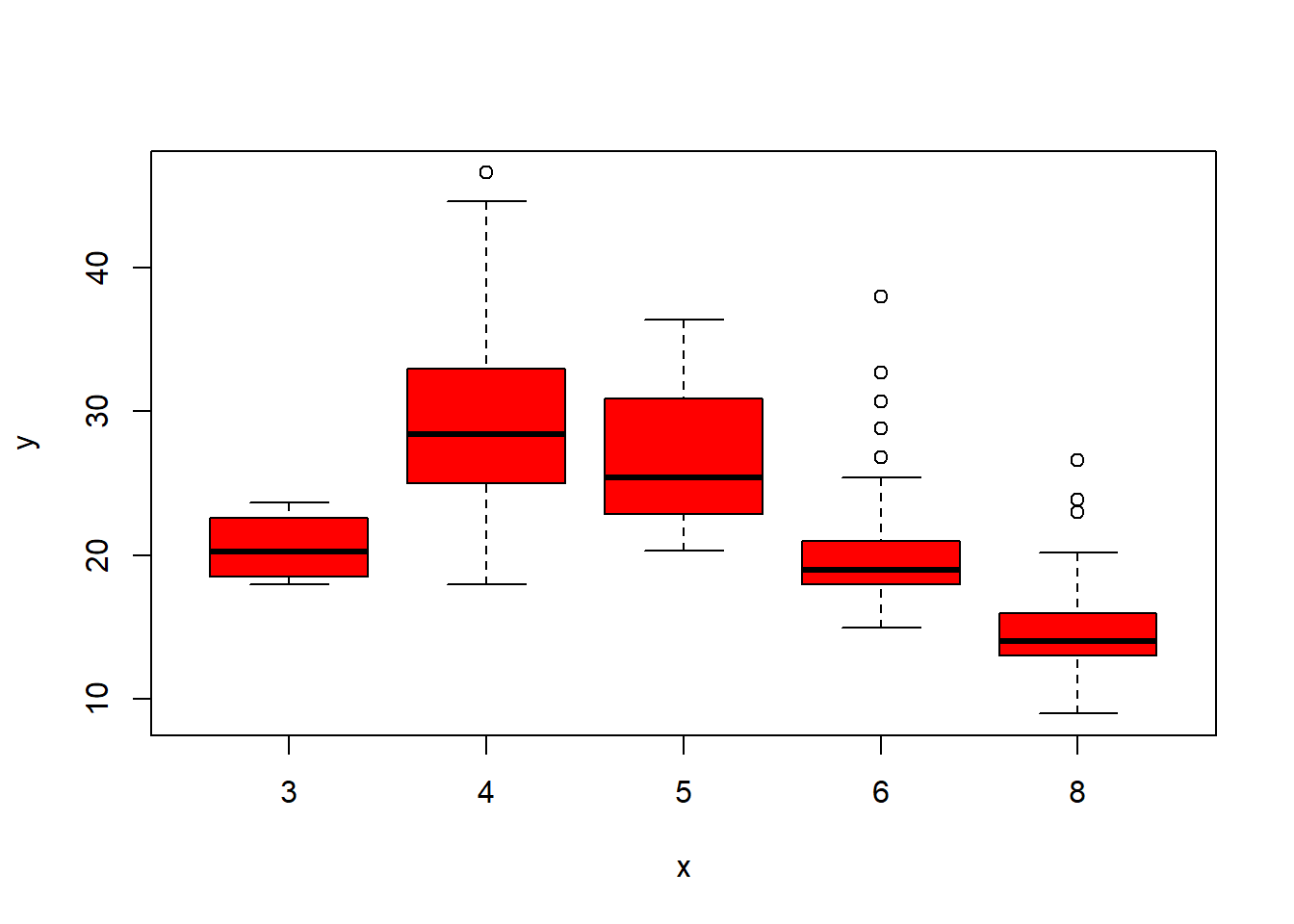
plot(cylinders, mpg, col="red", varwidth=T)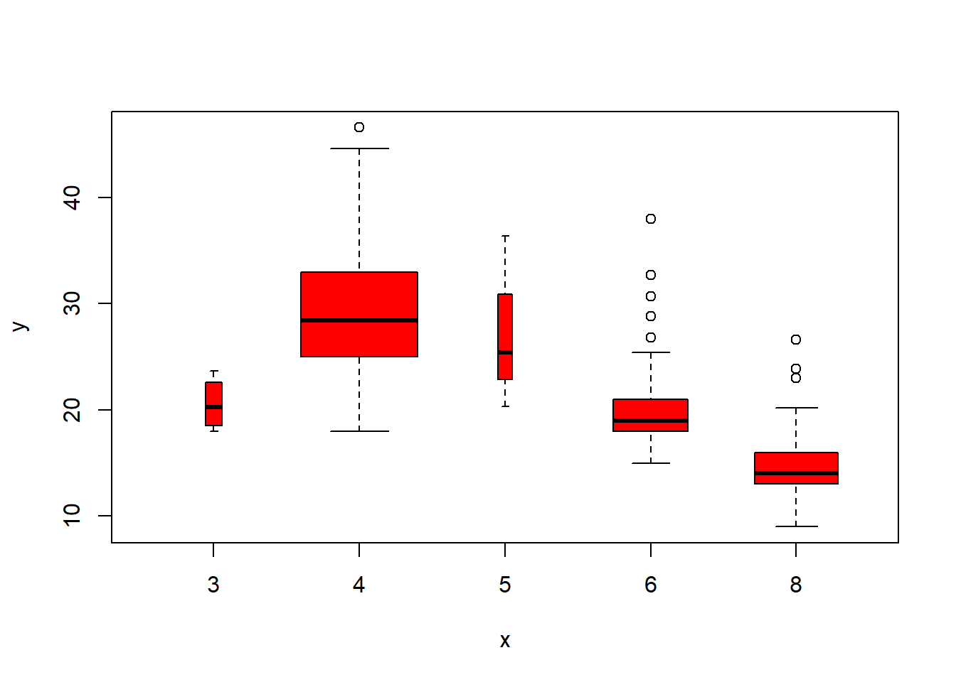
plot(cylinders, mpg, col="red", varwidth=T,horizontal=T)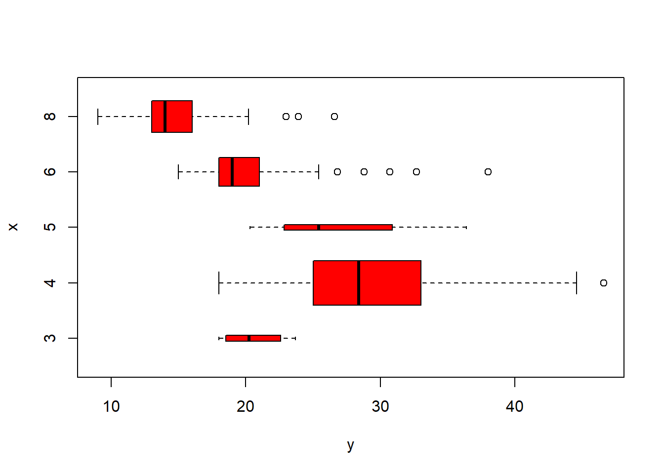
plot(cylinders, mpg, col="red", varwidth=T, xlab="cylinders", ylab="MPG")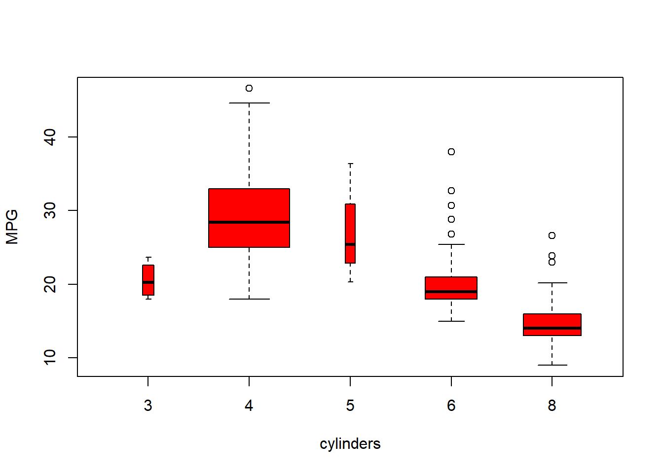
hist(mpg)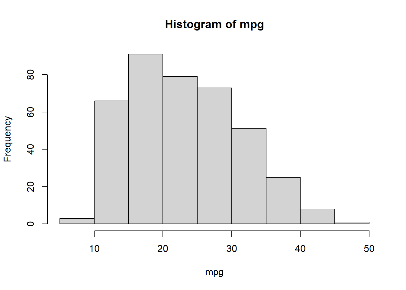
hist(mpg,col=2)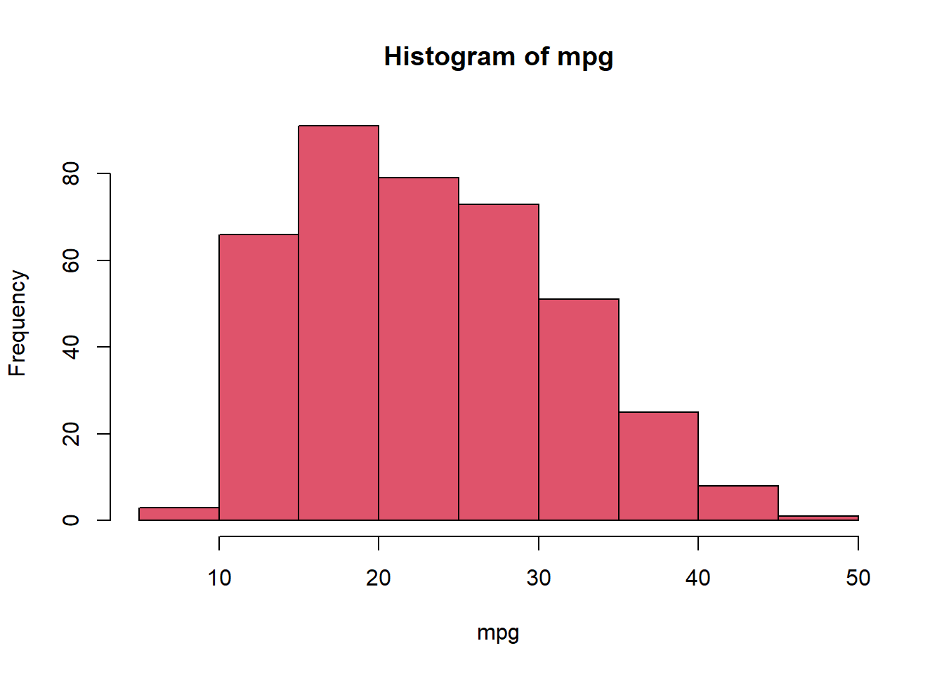
hist(mpg,col=2,breaks=15)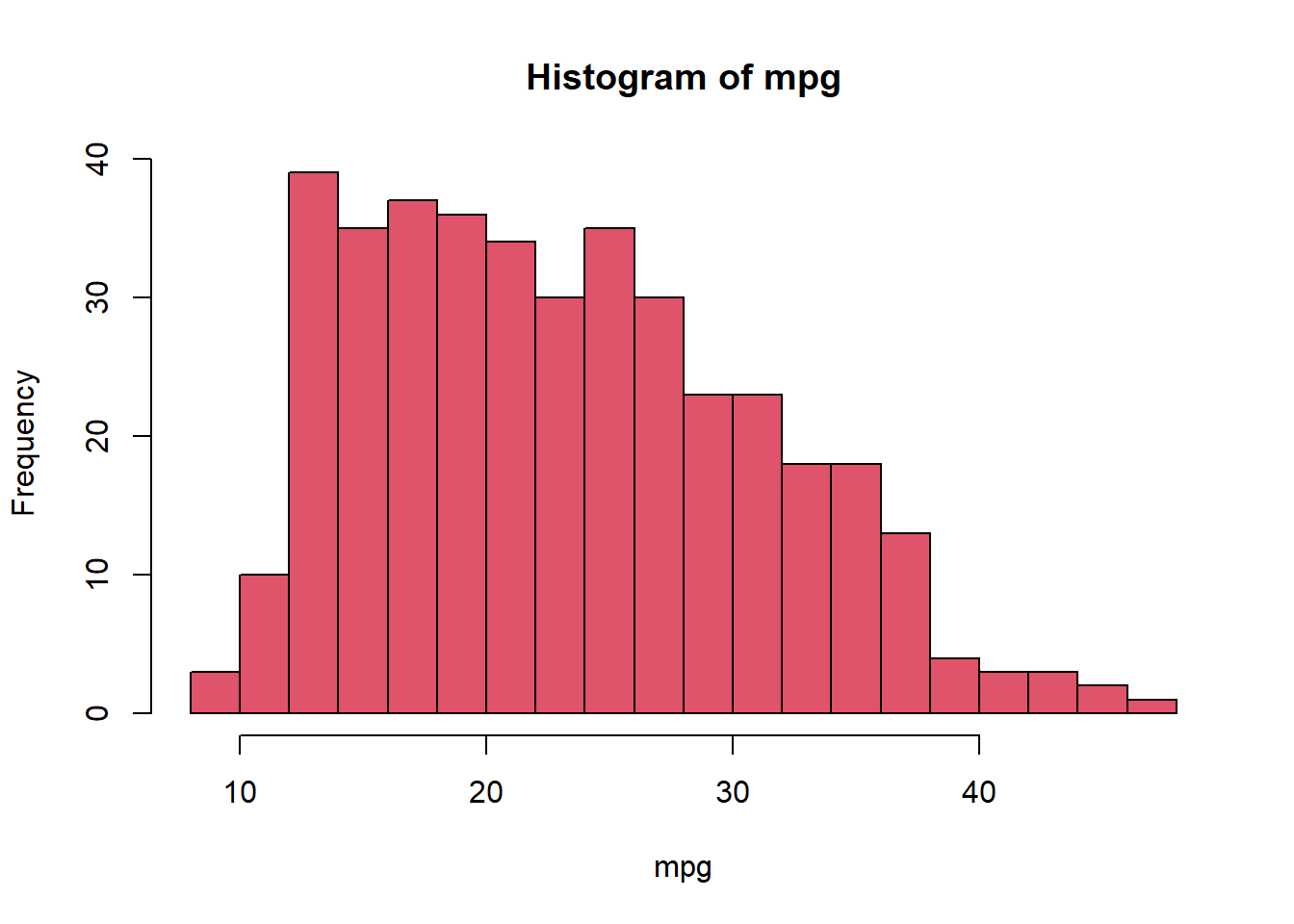
#pairs(Auto)
pairs(~ mpg + displacement + horsepower + weight + acceleration, Auto)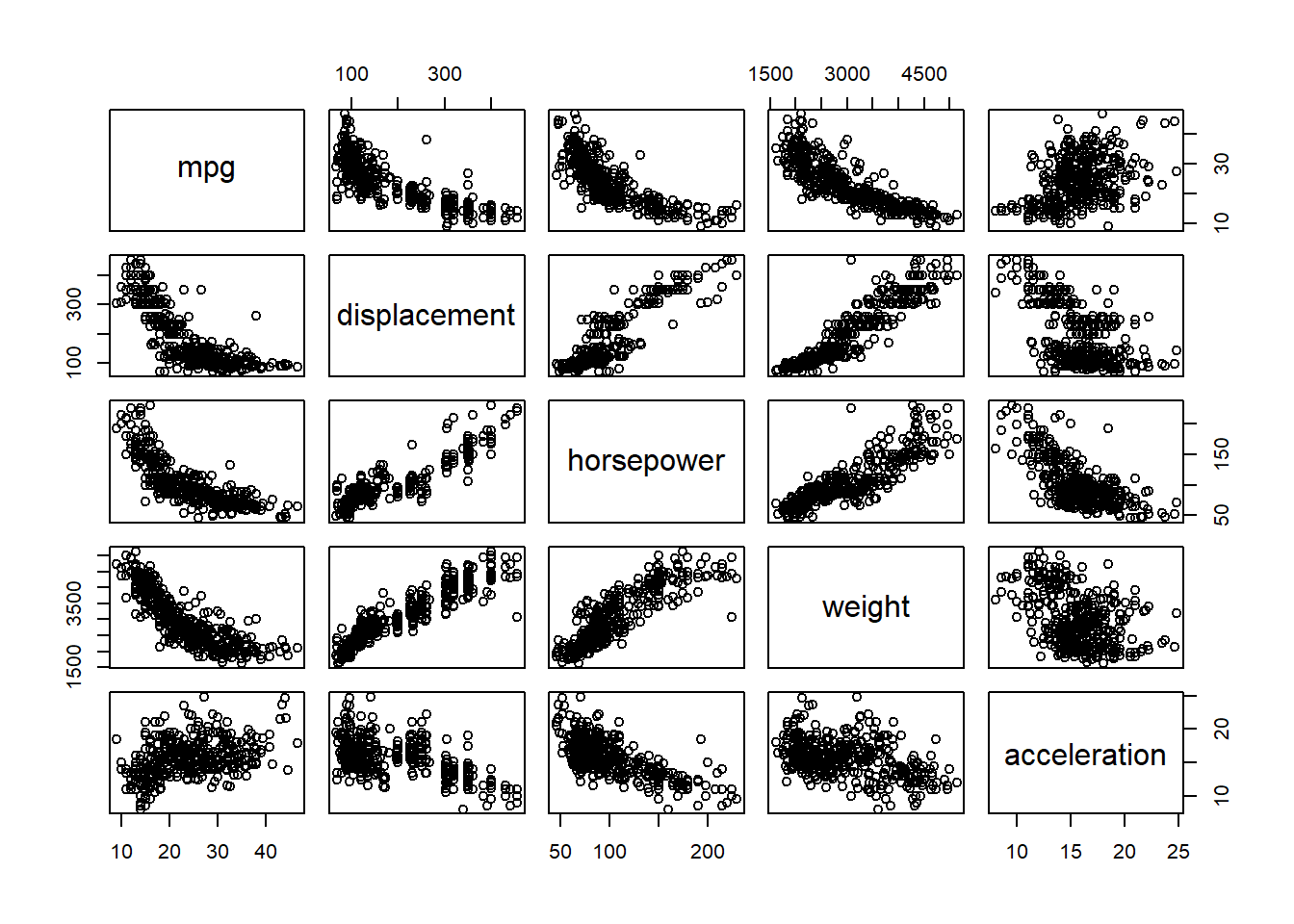
plot(horsepower,mpg)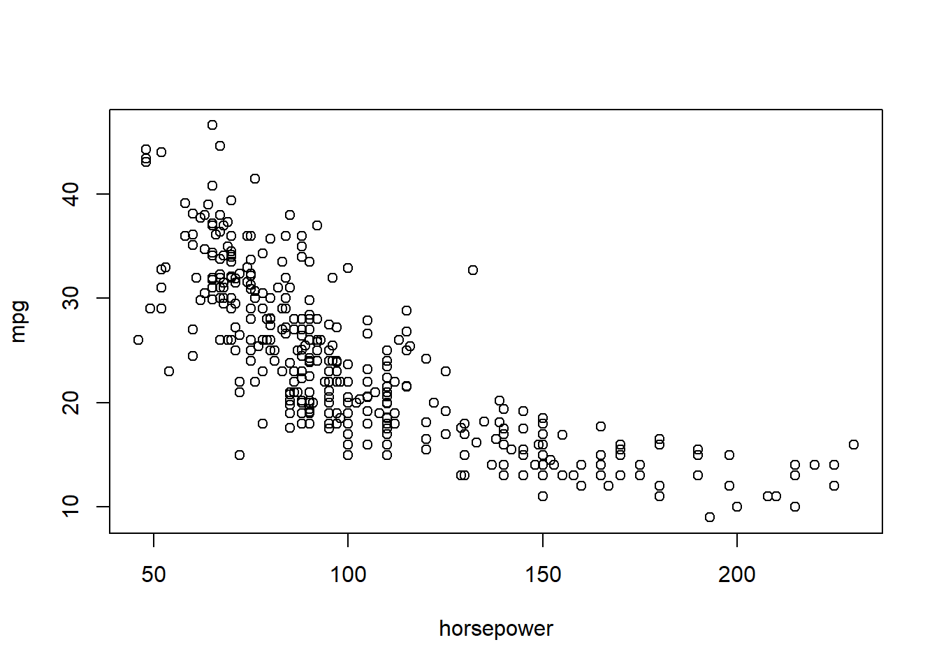
# identify(horsepower,mpg,name) # Interactive: point and click the dot to identify cases
summary(Auto)
mpg cylinders displacement horsepower weight
Min. : 9.00 Min. :3.000 Min. : 68.0 Min. : 46.0 Min. :1613
1st Qu.:17.50 1st Qu.:4.000 1st Qu.:104.0 1st Qu.: 75.0 1st Qu.:2223
Median :23.00 Median :4.000 Median :146.0 Median : 93.5 Median :2800
Mean :23.52 Mean :5.458 Mean :193.5 Mean :104.5 Mean :2970
3rd Qu.:29.00 3rd Qu.:8.000 3rd Qu.:262.0 3rd Qu.:126.0 3rd Qu.:3609
Max. :46.60 Max. :8.000 Max. :455.0 Max. :230.0 Max. :5140
NA's :5
acceleration year origin name
Min. : 8.00 Min. :70.00 Min. :1.000 Length:397
1st Qu.:13.80 1st Qu.:73.00 1st Qu.:1.000 Class :character
Median :15.50 Median :76.00 Median :1.000 Mode :character
Mean :15.56 Mean :75.99 Mean :1.574
3rd Qu.:17.10 3rd Qu.:79.00 3rd Qu.:2.000
Max. :24.80 Max. :82.00 Max. :3.000
summary(mpg) Min. 1st Qu. Median Mean 3rd Qu. Max.
9.00 17.50 23.00 23.52 29.00 46.60 ptbu=c("MASS","ISLR")
#install.packages(ptbu, repos='http://cran.us.r-project.org')
lapply(ptbu, require, character.only = TRUE)[[1]]
[1] TRUE
[[2]]
[1] TRUElibrary(MASS)
library(ISLR)
# Simple Linear Regression
# fix(Boston)
names(Boston) [1] "crim" "zn" "indus" "chas" "nox" "rm" "age"
[8] "dis" "rad" "tax" "ptratio" "black" "lstat" "medv" # lm.fit=lm(medv~lstat)
attach(Boston)
lm.fit=lm(medv~lstat,data=Boston)
attach(Boston)
lm.fit=lm(medv~lstat)
lm.fit
Call:
lm(formula = medv ~ lstat)

Coefficients:
(Intercept)        lstat
34.55 -0.95 summary(lm.fit)
Call:
lm(formula = medv ~ lstat)

Residuals:
    Min      1Q  Median      3Q     Max
-15.168  -3.990  -1.318   2.034  24.500

Coefficients:
            Estimate Std. Error t value Pr(>|t|)
(Intercept) 34.55384    0.56263   61.41   <2e-16 ***
lstat       -0.95005    0.03873  -24.53   <2e-16 ***
---
Signif. codes:  0 '***' 0.001 '**' 0.01 '*' 0.05 '.' 0.1 ' ' 1

Residual standard error: 6.216 on 504 degrees of freedom
Multiple R-squared:  0.5441,    Adjusted R-squared:  0.5432
F-statistic: 601.6 on 1 and 504 DF, p-value: < 2.2e-16names(lm.fit) [1] "coefficients" "residuals" "effects" "rank"
[5] "fitted.values" "assign" "qr" "df.residual"
[9] "xlevels" "call" "terms" "model" coef(lm.fit)(Intercept) lstat
34.5538409 -0.9500494 confint(lm.fit) 2.5 % 97.5 %
(Intercept) 33.448457 35.6592247
lstat -1.026148 -0.8739505predict(lm.fit,data.frame(lstat=(c(5,10,15))), interval="confidence") fit lwr upr
1 29.80359 29.00741 30.59978
2 25.05335 24.47413 25.63256
3 20.30310 19.73159 20.87461predict(lm.fit,data.frame(lstat=(c(5,10,15))), interval="prediction") fit lwr upr
1 29.80359 17.565675 42.04151
2 25.05335 12.827626 37.27907
3 20.30310 8.077742 32.52846# What is the differnce between "conference" and "prediction" difference?
plot(lstat,medv)
abline(lm.fit)
abline(lm.fit,lwd=3)
abline(lm.fit,lwd=3,col="red")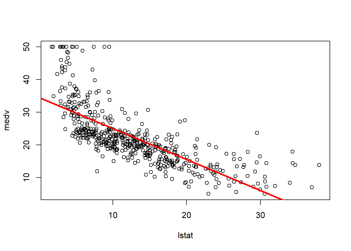
plot(lstat,medv,col="red")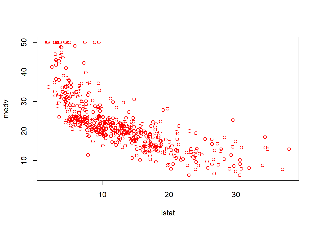
plot(lstat,medv,pch=16)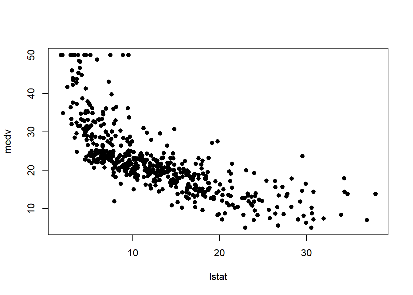
plot(lstat,medv,pch="+")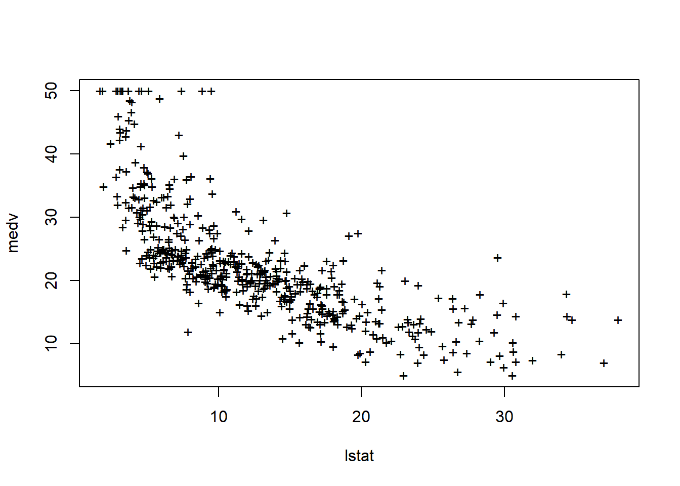
plot(1:20,1:20,pch=1:20)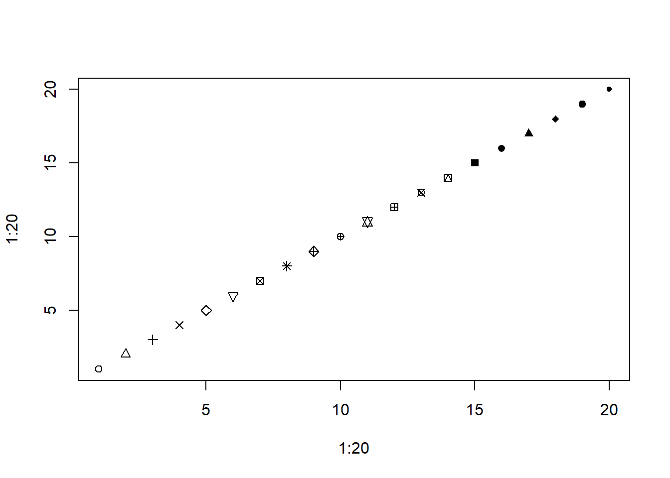
par(mfrow=c(2,2))
plot(lm.fit)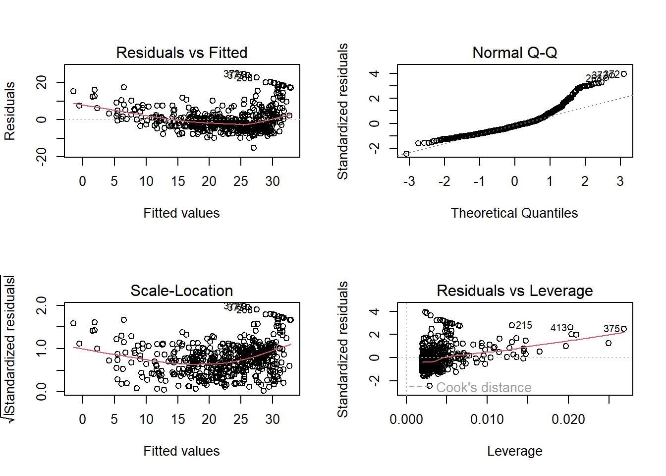
plot(predict(lm.fit), residuals(lm.fit))
plot(predict(lm.fit), rstudent(lm.fit))
plot(hatvalues(lm.fit))
which.max(hatvalues(lm.fit))
375
375 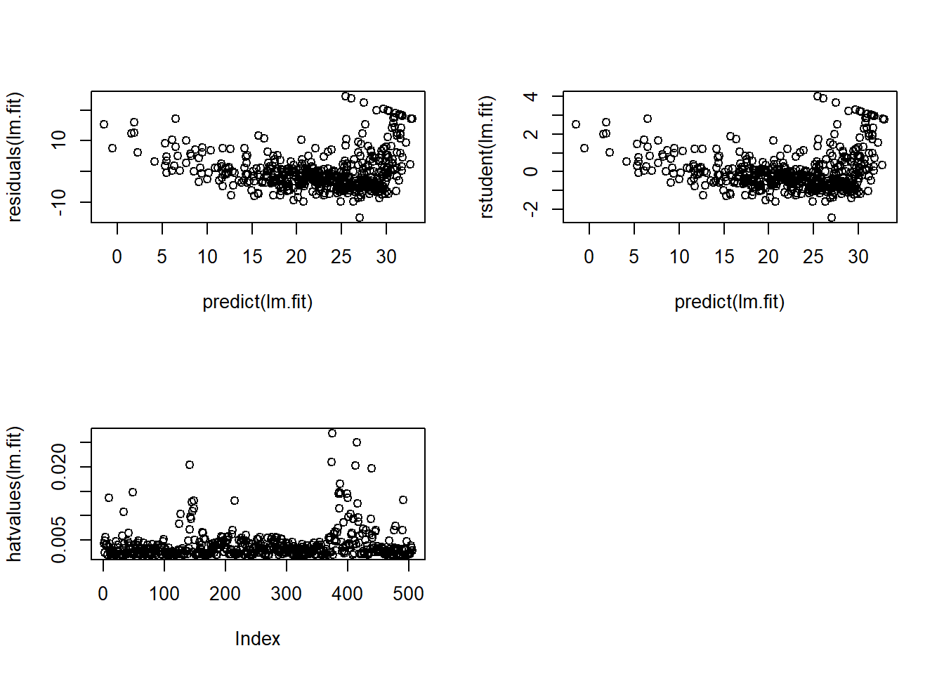
lm.fit=lm(medv~lstat+age,data=Boston)
summary(lm.fit)
Call:
lm(formula = medv ~ lstat + age, data = Boston)

Residuals:
    Min      1Q  Median      3Q     Max
-15.981  -3.978  -1.283   1.968  23.158

Coefficients:
            Estimate Std. Error t value Pr(>|t|)
(Intercept) 33.22276    0.73085  45.458  < 2e-16 ***
lstat       -1.03207    0.04819 -21.416  < 2e-16 ***
age          0.03454    0.01223   2.826  0.00491 **
---
Signif. codes:  0 '***' 0.001 '**' 0.01 '*' 0.05 '.' 0.1 ' ' 1

Residual standard error: 6.173 on 503 degrees of freedom
Multiple R-squared:  0.5513,    Adjusted R-squared:  0.5495
F-statistic: 309 on 2 and 503 DF, p-value: < 2.2e-16lm.fit=lm(medv~.,data=Boston)
summary(lm.fit)
Call:
lm(formula = medv ~ ., data = Boston)

Residuals:
    Min      1Q  Median      3Q     Max
-15.595  -2.730  -0.518   1.777  26.199

Coefficients:
              Estimate Std. Error t value Pr(>|t|)
(Intercept)  3.646e+01  5.103e+00   7.144 3.28e-12 ***
crim        -1.080e-01  3.286e-02  -3.287 0.001087 **
zn           4.642e-02  1.373e-02   3.382 0.000778 ***
indus        2.056e-02  6.150e-02   0.334 0.738288
chas         2.687e+00  8.616e-01   3.118 0.001925 **
nox         -1.777e+01  3.820e+00  -4.651 4.25e-06 ***
rm           3.810e+00  4.179e-01   9.116  < 2e-16 ***
age          6.922e-04  1.321e-02   0.052 0.958229
dis         -1.476e+00  1.995e-01  -7.398 6.01e-13 ***
rad          3.060e-01  6.635e-02   4.613 5.07e-06 ***
tax         -1.233e-02  3.760e-03  -3.280 0.001112 **
ptratio     -9.527e-01  1.308e-01  -7.283 1.31e-12 ***
black        9.312e-03  2.686e-03   3.467 0.000573 ***
lstat       -5.248e-01  5.072e-02 -10.347  < 2e-16 ***
---
Signif. codes:  0 '***' 0.001 '**' 0.01 '*' 0.05 '.' 0.1 ' ' 1

Residual standard error: 4.745 on 492 degrees of freedom
Multiple R-squared:  0.7406,    Adjusted R-squared:  0.7338
F-statistic: 108.1 on 13 and 492 DF, p-value: < 2.2e-16library(car)
vif(lm.fit) crim zn indus chas nox rm age dis
1.792192 2.298758 3.991596 1.073995 4.393720 1.933744 3.100826 3.955945
rad tax ptratio black lstat
7.484496 9.008554 1.799084 1.348521 2.941491 lm.fit1=lm(medv~.-age,data=Boston)
summary(lm.fit1)
Call:
lm(formula = medv ~ . - age, data = Boston)

Residuals:
     Min       1Q   Median       3Q      Max
-15.6054  -2.7313  -0.5188   1.7601  26.2243

Coefficients:
              Estimate Std. Error t value Pr(>|t|)
(Intercept)  36.436927   5.080119   7.172 2.72e-12 ***
crim         -0.108006   0.032832  -3.290 0.001075 **
zn            0.046334   0.013613   3.404 0.000719 ***
indus         0.020562   0.061433   0.335 0.737989
chas          2.689026   0.859598   3.128 0.001863 **
nox         -17.713540   3.679308  -4.814 1.97e-06 ***
rm            3.814394   0.408480   9.338  < 2e-16 ***
dis          -1.478612   0.190611  -7.757 5.03e-14 ***
rad           0.305786   0.066089   4.627 4.75e-06 ***
tax          -0.012329   0.003755  -3.283 0.001099 **
ptratio      -0.952211   0.130294  -7.308 1.10e-12 ***
black         0.009321   0.002678   3.481 0.000544 ***
lstat        -0.523852   0.047625 -10.999  < 2e-16 ***
---
Signif. codes:  0 '***' 0.001 '**' 0.01 '*' 0.05 '.' 0.1 ' ' 1

Residual standard error: 4.74 on 493 degrees of freedom
Multiple R-squared:  0.7406,    Adjusted R-squared:  0.7343
F-statistic: 117.3 on 12 and 493 DF, p-value: < 2.2e-16lm.fit1=update(lm.fit, ~.-age)lm.fit2=lm(medv~lstat+I(lstat^2))
summary(lm.fit2)
Call:
lm(formula = medv ~ lstat + I(lstat^2))

Residuals:
     Min       1Q   Median       3Q      Max
-15.2834  -3.8313  -0.5295   2.3095  25.4148

Coefficients:
             Estimate Std. Error t value Pr(>|t|)
(Intercept) 42.862007   0.872084   49.15   <2e-16 ***
lstat       -2.332821   0.123803  -18.84   <2e-16 ***
I(lstat^2)   0.043547   0.003745   11.63   <2e-16 ***
---
Signif. codes:  0 '***' 0.001 '**' 0.01 '*' 0.05 '.' 0.1 ' ' 1

Residual standard error: 5.524 on 503 degrees of freedom
Multiple R-squared:  0.6407,    Adjusted R-squared:  0.6393
F-statistic: 448.5 on 2 and 503 DF, p-value: < 2.2e-16lm.fit=lm(medv~lstat)
anova(lm.fit,lm.fit2)Analysis of Variance Table
Model 1: medv ~ lstat
Model 2: medv ~ lstat + I(lstat^2)
Res.Df RSS Df Sum of Sq F Pr(>F)
1 504 19472
2 503 15347 1 4125.1 135.2 < 2.2e-16 ***
---
Signif. codes: 0 '***' 0.001 '**' 0.01 '*' 0.05 '.' 0.1 ' ' 1par(mfrow=c(2,2))
plot(lm.fit2)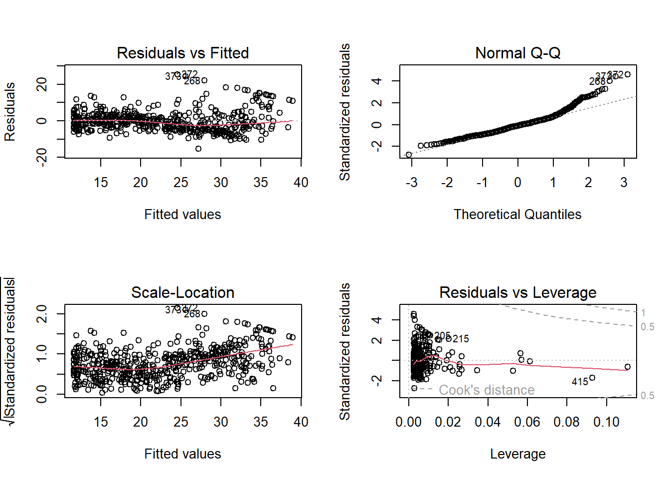
lm.fit5=lm(medv~poly(lstat,5))
summary(lm.fit5)
Call:
lm(formula = medv ~ poly(lstat, 5))

Residuals:
     Min       1Q   Median       3Q      Max
-13.5433  -3.1039  -0.7052   2.0844  27.1153

Coefficients:
                 Estimate Std. Error t value Pr(>|t|)
(Intercept)       22.5328     0.2318  97.197  < 2e-16 ***
poly(lstat, 5)1 -152.4595     5.2148 -29.236  < 2e-16 ***
poly(lstat, 5)2   64.2272     5.2148  12.316  < 2e-16 ***
poly(lstat, 5)3  -27.0511     5.2148  -5.187 3.10e-07 ***
poly(lstat, 5)4   25.4517     5.2148   4.881 1.42e-06 ***
poly(lstat, 5)5  -19.2524     5.2148  -3.692 0.000247 ***
---
Signif. codes:  0 '***' 0.001 '**' 0.01 '*' 0.05 '.' 0.1 ' ' 1

Residual standard error: 5.215 on 500 degrees of freedom
Multiple R-squared:  0.6817,    Adjusted R-squared:  0.6785
F-statistic: 214.2 on 5 and 500 DF, p-value: < 2.2e-16summary(lm(medv~log(rm),data=Boston))
Call:
lm(formula = medv ~ log(rm), data = Boston)

Residuals:
    Min      1Q  Median      3Q     Max
-19.487  -2.875  -0.104   2.837  39.816

Coefficients:
            Estimate Std. Error t value Pr(>|t|)
(Intercept)  -76.488      5.028  -15.21   <2e-16 ***
log(rm)       54.055      2.739   19.73   <2e-16 ***
---
Signif. codes:  0 '***' 0.001 '**' 0.01 '*' 0.05 '.' 0.1 ' ' 1

Residual standard error: 6.915 on 504 degrees of freedom
Multiple R-squared:  0.4358,    Adjusted R-squared:  0.4347
F-statistic: 389.3 on 1 and 504 DF, p-value: < 2.2e-16# fix(Carseats)
names(Carseats) [1] "Sales" "CompPrice" "Income" "Advertising" "Population"
[6] "Price" "ShelveLoc" "Age" "Education" "Urban"
[11] "US" lm.fit=lm(Sales~.+Income:Advertising+Price:Age,data=Carseats)
summary(lm.fit)
Call:
lm(formula = Sales ~ . + Income:Advertising + Price:Age, data = Carseats)

Residuals:
    Min      1Q  Median      3Q     Max
-2.9208 -0.7503  0.0177  0.6754  3.3413

Coefficients:
                     Estimate Std. Error t value Pr(>|t|)
(Intercept)         6.5755654  1.0087470   6.519 2.22e-10 ***
CompPrice           0.0929371  0.0041183  22.567  < 2e-16 ***
Income              0.0108940  0.0026044   4.183 3.57e-05 ***
Advertising         0.0702462  0.0226091   3.107 0.002030 **
Population          0.0001592  0.0003679   0.433 0.665330
Price              -0.1008064  0.0074399 -13.549  < 2e-16 ***
ShelveLocGood       4.8486762  0.1528378  31.724  < 2e-16 ***
ShelveLocMedium     1.9532620  0.1257682  15.531  < 2e-16 ***
Age                -0.0579466  0.0159506  -3.633 0.000318 ***
Education          -0.0208525  0.0196131  -1.063 0.288361
UrbanYes            0.1401597  0.1124019   1.247 0.213171
USYes              -0.1575571  0.1489234  -1.058 0.290729
Income:Advertising  0.0007510  0.0002784   2.698 0.007290 **
Price:Age           0.0001068  0.0001333   0.801 0.423812
---
Signif. codes:  0 '***' 0.001 '**' 0.01 '*' 0.05 '.' 0.1 ' ' 1

Residual standard error: 1.011 on 386 degrees of freedom
Multiple R-squared:  0.8761,    Adjusted R-squared:  0.8719
F-statistic: 210 on 13 and 386 DF, p-value: < 2.2e-16attach(Carseats)
contrasts(ShelveLoc) Good Medium
Bad 0 0
Good 1 0
Medium 0 1summary(lm(medv~lstat*age,data=Boston))
Call:
lm(formula = medv ~ lstat * age, data = Boston)

Residuals:
    Min      1Q  Median      3Q     Max
-15.806  -4.045  -1.333   2.085  27.552

Coefficients:
              Estimate Std. Error t value Pr(>|t|)
(Intercept) 36.0885359  1.4698355  24.553  < 2e-16 ***
lstat       -1.3921168  0.1674555  -8.313 8.78e-16 ***
age         -0.0007209  0.0198792  -0.036   0.9711
lstat:age    0.0041560  0.0018518   2.244   0.0252 *
---
Signif. codes:  0 '***' 0.001 '**' 0.01 '*' 0.05 '.' 0.1 ' ' 1

Residual standard error: 6.149 on 502 degrees of freedom
Multiple R-squared:  0.5557,    Adjusted R-squared:  0.5531
F-statistic: 209.3 on 3 and 502 DF,  p-value: < 2.2e-16